Oilfield ESP economics: water cut changes the oil-cost denominator
A hydraulic-duty model shows why a stable electricity bill can conceal rising lifting cost per unit of oil.
AI-generated editorial illustration; it does not depict a verified project, actual prices or chart data.
1. The bill can stay flat while oil gets expensive
An electric submersible pump lifts liquid, not only saleable oil. If water replaces oil at unchanged liquid throughput, the same electricity expense is divided by less oil. That denominator effect can dominate a small tariff movement. The decision is therefore not simply whether to purchase a more efficient motor. It is whether the complete lift and water-handling system produces incremental oil margin after electricity, treatment, disposal and reliability costs.
2. The dated energy context
The October 6 EIA outlook, finalized October 1, forecasts 2026 US wholesale electricity at 52 USD/MWh. That is neither a delivered oilfield tariff nor an observed October average. The World Bank October 2 release records Brent at 90.9 USD/bbl in August and 116.8 in September. A benchmark crude price is not the well's realized netback: quality differential, transportation and contract terms remain. Neither source supplies a verified August/September ESP service quotation used here.
3. Hydraulic mechanism and its limits
For a simplified incompressible duty, electrical power is density × gravity × volumetric flow × head / overall wire-to-fluid efficiency. Flow must be in m³/s and the result is watts. Head means total differential head, including pressure and friction requirements; it is not automatically equal to pump setting depth. Gas, viscosity, emulsion, changing density, solids and reservoir inflow can invalidate a simple fixed-head comparison. SLB's technical discussion describes how changing water/gas cut and reservoir conditions affect ESP operation. The model below intentionally holds those effects fixed to isolate dilution of oil output.
4. Illustrative daily calculation
Assume liquid flow 1000 m³/day, density 1000 kg/m³, total head 1500 m, gravity 9.81 m/s², overall efficiency 0.60 and electricity 100 USD/MWh. These are hypothetical nominal USD assumptions excluding tax. Power = 1000 × 9.81 × (1000 / 86400) × 1500 / 0.60 / 1000 = 283.85417 kW. Daily energy is 6812.5 kWh before rounding. For the following cost model use the rounded engineering duty 283.85 kW, giving 6812.4 kWh/day and 681.24 USD/day consistently.
| Daily item | Calculation | Result |
|---|---|---|
| Electrical duty | Rounded hydraulic calculation | 283.85 kW |
| Electricity | 283.85 × 24 | 6812.4 kWh |
| Electricity expense | 6812.4 / 1000 × 100 | 681.24 USD |
| Oil at 80% water | 1000 × (1 − 0.80) | 200 m³ |
| Cost per oil volume | 681.24 / 200 | 3.4062 USD/m³ |
The cost includes lift electricity only. Separate water separation, injection, chemicals, workovers, fixed labor, royalties and capital recovery. Production volumes must refer to the same measurement conditions; do not divide downhole liquid flow by surface oil volume without the appropriate volume reconciliation.
5. Water-cut sensitivity
At 50%, 80% and 90% water, oil volumes are 500, 200 and 100 m³/day. Lift electricity cost becomes 1.36248, 3.4062 and 6.8124 USD/m³ oil. Moving from 80% to 90% doubles this unit cost without increasing the modeled bill. A 20 USD/MWh tariff increase adds 136.248 USD/day, or 0.68124 USD/m³ at 80% water. If overall efficiency falls from 60% to 50%, energy rises by 20% at unchanged hydraulic work; this is distinct from the water denominator effect.
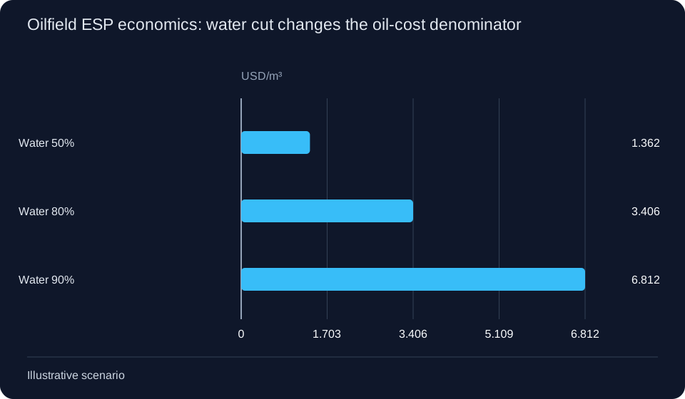
Illustrative electricity cost per m³ oil at water cuts 50%, 80% and 90%; liquid flow 1000 m³/day, density 1000 kg/m³, head 1500 m, efficiency 60% and power 100 USD/MWh are fixed. This isolates the denominator, not a well forecast.
| Water cut | Oil m³/day | Electricity USD/m³ oil |
|---|---|---|
| 50% | 500 | 1.36248 |
| 80% | 200 | 3.4062 |
| 90% | 100 | 6.8124 |
6. Operating and contract decisions
Require synchronized measurements of liquid, oil, water, input kW, pump intake/discharge pressure, speed and availability. Compare specific energy at matched duty before attributing a change to efficiency. Request pump curves, gas-handling limits, cable and transformer losses, harmonics and restart constraints. Do not reduce speed from an energy calculation alone: minimum flow for cooling, stable reservoir operation and production targets still apply. Water-reduction interventions deserve evaluation when avoided disposal and lift expense exceed intervention cost without sacrificing profitable oil.
7. Questions and boundaries
Does high water cut prove the ESP should stop? No. Compare incremental oil netback with avoidable lift and water costs, including restart risk and reservoir obligations.
Can pump depth replace head? No. Use differential pressure, fluid properties and system losses; reservoir pressure can supply part of the lift.
Can tariff forecasts justify a motor replacement? Not alone. Measured efficiency, operating hours, workover cost and expected service life determine whether savings can recover the investment.
8. Sources and next decisions
Use EIA forecast timing, World Bank crude context, SLB ESP mechanism and DOE system matching within their scope. Continue to the industrial bill guide and dewatering hydraulic model. Use the ROI calculator only after including workover and downtime boundaries.
- Industrial Electricity Bills: Energy, Network and Demand Costs in 2026
- EU–US Industrial Power Prices: Match Tax, Currency and Delivery Basis
- Natural Gas and LNG: From Hub Benchmark to Delivered Industrial Cost
- Brent, WTI and Refinery Energy Costs: A Margin Scenario Bridge
- Transformer Procurement: A Copper, Aluminium, Oil and Currency Cost Bridge
- Copper and Aluminium Winding Costs: Metal Pass-Through and Indexation in 2026
- GOES Electrical Steel Economics: Yield, Loss and Grade Premium in 2026
- Mineral Oil versus Natural Ester: Transformer Life-Cycle Cost Boundaries in 2026
- Lithium, Nickel and Graphite Exposure: Battery Procurement Cost Bridges in 2026
- Recycled Copper Economics: Quality, Recovery Yield and Energy Cost in 2026
- Transformer landed cost: Incoterms, ocean freight, road delivery and insurance in 2026
- Transformer heavy haul: route, permits, storage and remobilization costs
- LNG shipping economics: freight, boil-off and delivered energy cost
- Port delay economics: working capital, storage and equipment demurrage
- Diesel and bunker freight surcharges: an auditable indexation model
- Solar LCOE: Financing, Curtailment and Interconnection in 2026
- Wind Capture Price: Congestion, Export Losses and Revenue
- BESS Arbitrage: Throughput, Degradation and Net Spread
- Industrial Power PPAs: Fixed, Floating and Profile Risk
- Transformer Losses: Capital Premium, Electricity Cost and NPV
- Refinery hydrogen: separate gas, electricity and carbon costs
- LNG liquefaction: electric-drive versus gas-turbine energy cost
- Oilfield ESP economics: water cut changes the oil-cost denominator
- Gas-generator spark spread: net heat rate turns fuel into cost
- Liquid-pipeline pumping: electricity versus diesel cost scenarios
- Copper Mine Energy Cost: Grade and Recovery Matter More Than a Headline Tariff
- SAG Mill Economics: Lower kWh/t Must Preserve Throughput and Recovery
- Mine Conveyor or Haul Trucks: Energy Prices and the Throughput Break-Even
- Mine Dewatering Cost: Total Head and Wire-to-Water Efficiency
- Mine Power Reliability: Value Outage Hours, Restart Losses and Backup Costs Separately
- SFRA After Transformer Transport: Distinguishing Winding Movement from a Changed Setup
- Transformer Moisture: Why the Same ppm Means Different Risk in Mineral Oil and Ester
- Bushing Capacitance and tan δ: Build a Temperature-Consistent Trend Before Replacement
- OLTC Dynamic Resistance: Diagnose Transition-Resistor Signatures Without False Alarms
- Transformer Winding Resistance: Correct Temperature Before Comparing Phases and Factory Data
- Restricted Earth Fault: Proving the Transformer Neutral CT Zone
- GOOSE with PRP or HSR: Supervise the Trip, Not Just the Link
- 1 A or 5 A CT Secondaries: Calculate the Long-Cable Burden
- MV Breaker Failure 50BF: Build the Timer and Intertrip Budget
- NGR Continuity Monitoring: Respond to an Open or Bypassed Resistor
- BESS Transformer RFQs: Evaluate Losses Against the Actual Duty Cycle
- MV Collector Protection When Inverter Fault Current Barely Exceeds Load
- Grid-Forming BESS Black Start: Prove Transformer Energization Before Load Pickup
- Dual-LV Solar Transformers: Specify Every Pairwise Impedance and Its Base
- Renewable Collector Harmonic Scans: Include Cable Capacitance and Converter Impedance
- Refinery Voltage-Sag Ride-Through: Coordinating VFDs, Contactors and Process Permissives
- LNG Compressor Starting: A Transformer Study for Voltage Dip and Acceleration
- ESP Drives, Step-Up Transformers and Long Cables: Separating Resonance from Voltage Drop
- Pressurized Electrical Rooms in Hazardous Areas: Purge, Pressure-Loss and Trip Interfaces
- Refinery UPS Selectivity: Static Bypass, Inverter Limits and Branch Fault Clearing
- Underground Trailing Cables: Coordinate Ground Check and Neutral Protection
- Downhill Conveyor Regeneration: Specify the Transformer and Grid Interface
- Mine Hoist Transformers: Use RMS Cycle Screening Without Hiding Hot Spots
- SAG Mill Drive Transformers: Coordinate Harmonics, Filters and Network Impedance
- High-Altitude Mining Transformers: Separate Clearance and Cooling Guarantees
- Short-Circuit Test Reports: Proving Similarity to the Offered Transformer
- Transformer Noise Guarantees: Sound Power, Sound Pressure and Acceptance
- Ester Retrofill Review: Gaskets, OLTC Approval and the Remaining Mineral Oil
- Reusing a 50/60 Hz Transformer: V/Hz Is Only the First Check
- EU F-Gas Switchgear Procurement in 2026: Rated Voltage and Evidence Scope
- Ecodesign Tier 2 Transformer Standards: No-Load and Load-Loss Limits
- No-Load Loss (P0) Reduction Physics: Laser-Scribed CRGO vs Amorphous Alloy Cores
- Transformer Load Loss (Pk) Optimization: CTC Conductors and Stray Loss Mitigation
- Cast Resin Dry-Type vs Liquid-Immersed Transformers: Selection Guide
- Forced Air (AF) Cooling Dynamics in Cast Resin Transformers: +40% Power Uprating
- Partial Discharge (PD) Testing and Diagnostics in Cast Resin Transformers
- Ester Dielectric Fluids in Power Transformers: Natural vs Synthetic Esters vs Mineral Oil
- Transformer Thermal Modeling and Winding Hot-Spot Calculation (IEC 60076-2 / IEC 60076-7)
- Conservator Preservation Systems, Buchholz Relays, and DGA Duval Triangle Diagnostics
- Step-Up Transformer Engineering for Utility Solar PV, Wind and BESS Plants
- Wind Turbine Nacelle and Tower Transformers: 3G Vibration and Marine Corrosion Design
- BESS Battery Energy Storage Coupling Transformers: Four-Quadrant P-Q Operation and dV/dt Stresses
- Substation Step-Down Power Transformers (110 kV to 330 kV): Design & OLTC Regulation
- On-Load Tap Changer (OLTC) Vacuum Technology and Automatic Voltage Regulation (AVR)
- Ultra-High Voltage (UHV 1000 kV) Transformers and SCB18 Dry-Type Technology
- Generator Step-Up (GSU) Transformers: Saturation, Overfluxing (V/Hz), and Tertiary Stabilizing Windings
- Heavy Industry Process Transformers: Electric Arc Furnace (EAF) & Green Hydrogen Rectifiers
- Variable Frequency Drive (VFD) Multi-Pulse Isolation Transformers: Harmonic Cancellation
- Grounding Transformers (Zigzag ZN) and Neutral Earthing Resistors (NGR): Sizing & Fault Duty
- Medium Voltage Switchgear Selection: Air-Insulated (AIS) vs Gas-Insulated (GIS)
- Vacuum Circuit Breaker (VCB) Switching Dynamics: Transient Recovery Voltage (TRV) and RC Snubbers
- Ring Main Units (RMU) for Secondary Distribution: Architecture, CCF Topologies, and Telemetry Automation
- Transformer Differential Protection (ANSI 87T): Biased Slope, Inrush Restraint, and CT Saturation
- IEC 61850 Substation Automation: GOOSE Messaging, Sampled Values (SV), and Process Bus Protection
- Prefabricated and Pad-Mounted Substations: IEC 62271-202 Selection Guide
- Diesel and Gas Generator Sets: ISO 8528 Rating and Selection Guide
- Instrument Transformers: CT and VT Selection for Metering and Protection
- Surge Arresters and Insulation Coordination: IEC 60099-4 / IEC 60071 Guide
- Power Quality and Reactive Compensation: Capacitor Banks, SVC and STATCOM
- Medium-Voltage Cables and Busways: Ampacity, Voltage Drop and Short-Circuit Selection
- Industrial Motor Selection: IEC 60034 Ratings, Starting and IE Efficiency
- UPS, BESS and Critical Power: Autonomy, Topology and Safety Selection
- Transformer FAT and Site Commissioning: IEC 60076 Test Plan
- Mobile Emergency Substations: Rapid Deployment and Interface Selection
- Rail Traction Transformers: AC/DC Supply, Regeneration and Vibration Duty
- Shore Power Transformers: IEC/IEEE 80005-1 HVSC Interface Design
- Mining and Flameproof Transformers: Ex-Zone, Cooling and Protection Selection
- LV Power Switchboards: IEC 61439 Design Verification and Assembly Data
- LV Breakers, Switches, Fuses and Contactors: IEC 60947 Coordination
- Automatic Reclosers and Feeder Automation: IEC 62271-111 Selection
- MV Feeder Protection Settings: 50/51, 67, 79 and IEC 60255 Evidence
- Generator ATS, AMF and Paralleling: ISO 8528 and IEC 60947-6-1
- Power Meters and Power-Quality Monitoring: IEC 61557-12 / 61000-4-30
- PV Inverter Grid Connection: Anti-Islanding, Reactive Power and Transformer Interface
- EV Charging Infrastructure: Transformer Sizing, Protection and IEC 61851
- Pad-Mounted Transformers: Dead-Front Loop-Feed Design, Fusing and IEEE C57.12.26
- Monoblock Concrete Substations: Internal Arc (IAC-AB), Ventilation and IEC 62271-202
- Biogas and Landfill CHP Gensets: Fuel Gas Treatment, Methane Number and ISO 8528
- Synchronous Generator Protection and Grid Code Compliance: ANSI 32, 40, 46, 81 and FRT
- Electrostatic Shielded Solar Transformers: Inverter Harmonics, K-Factor and Ester Oil
- Busbar Differential Protection (ANSI 87B): High-Impedance vs Distributed Numerical Architecture
- Transmission Autotransformers: Delta Tertiary Stabilization, Zero-Sequence Impedance and Sizing
- Amorphous Metal Core Transformers: Fe-Si-B Ribbon Physics, Acoustic Design and Life-Cycle TOC
- Subsurface and Vault-Mounted Distribution Transformers: Flood Protection and IEEE C57.12.40
- Emergency Diesel Generator Fast-Starting: ISO 8528-5 Class G3 Dynamics and NFPA 110
- Submerged Arc Furnace (SAF) Transformers: High-Current Secondary Bus Electrodynamics
- Floating Solar PV (FPV) Transformer Substations: Marine Corrosion, Buoyancy and Tilt
- ETAP Alternative for Single Line Diagrams: A Practical Selection Guide
- How to Create an Electrical Single Line Diagram Online
- Single Line Diagram vs Load-Flow Model: Validation Before Analysis