Load Flow Analysis Explained: AC, DC and a Reproducible Two-Bus Example
Understand AC load-flow equations, distinguish two DC models, and reproduce a two-bus solution with explicit units, power balance and engineering limits.
AI-generated editorial illustration. Not a manufacturer photograph, real project, engineering diagram or simulated result.
1. What does load flow calculate?
Load flow, or power flow, calculates a network's steady-state bus voltages, branch currents, power transfers and losses for a declared operating condition. It answers whether the specified injections and controls produce an acceptable operating point. It does not calculate fault withstand, relay selectivity, motor acceleration or transient stability merely because those components appear on a single-line diagram. Those questions need different data and studies.
Electrical Analysis is Voltformer's primary engineering workspace. Its connected SLD provides equipment identities and topology; the selected study provides mathematical assumptions. This guide develops an independently reproducible two-bus example and explains how to use it as a small acceptance case. All example inputs are assumed educational values, not manufacturer data or a proposed installation. Reviewed 12 November 2026.
2. Start with a model contract
Record the system frequency, voltage and MVA bases, energized topology, slack source voltage, branch impedances, transformer tap orientation, load demand and generator controls. State whether branch data are in ohms, ohms per kilometre, percent or per unit. A cable resistance per kilometre becomes an impedance only after its length and parallel arrangement are applied. A three-phase load in MW is not a per-phase load.
For balanced three-phase quantities, Zbase = Vbase,LL² / Sbase,3φ. Consistent kV and MVA give ohms. The per-unit impedance is Zohm / Zbase. When changing bases, Zpu,new = Zpu,old × (Snew/Sold) × (Vold/Vnew)². Record the reference side of every transformer impedance. A nominal ratio and an off-nominal tap perform different functions in the network model.
Classify input evidence before solving: Manufacturer Verified applies only to the identified document and configuration; Engineering Derived identifies the equation and parent inputs; User Supplied identifies project information; Assumed identifies a study scenario; Unknown means evidence is missing. Copying a catalog family value into a project does not upgrade its evidence status. Save the selected record revision so a later catalog edit cannot silently change the case.
3. AC equations and bus types
At each bus, Inet = Ybus V and Sinjection = V × conjugate(Inet). A positive net injection denotes generation; positive demand must therefore enter an injection formulation with the opposite sign. Use one sign convention throughout the dataset, report and independent check.
A slack bus fixes voltage magnitude and angle while balancing the remaining real and reactive mismatch. A PQ bus specifies net P and Q. A PV bus specifies P and voltage magnitude; Q becomes an output until a declared reactive limit requires a different operating mode. An iterative solver's convergence flag establishes only its stated numerical residual, not compliance with equipment or utility limits. Also inspect the accepted bus types, control positions and warnings.
The MATPOWER manual documents these bus distinctions and the nonlinear AC problem. Voltformer's current balanced solver is Newton–Raphson; separately entered ABC models, resistive DC models and other network studies have their own input boundaries. A balanced result cannot establish neutral loading or phase unbalance.
4. A two-bus case with an independent closed form
Assume a 1 MVA, 11 kV line-to-line base, slack E = 1 + j0 pu, a series branch Z = 0.05 + j0.10 pu, and a receiving load S = 0.50 + j0.20 pu. Omit shunt admittance, taps and other injections. These are deliberately simple assumptions. The corresponding base impedance is 121 Ω; the branch is 6.05 + j12.10 Ω and the three-phase load is 0.50 MW + j0.20 Mvar.
Let x = |V|², a = RP + XQ = 0.045 and b = (R² + X²)(P² + Q²) = 0.003625. From S = V × conjugate((E − V)/Z), with E = 1, obtain x² + (2a − 1)x + b = 0. The higher-voltage root gives x = 0.905998891351. Recover V = x + a − j(XP − RQ) = 0.950998891351 − j0.04 pu.
The load-bus magnitude is 0.951839740372 pu, its angle is −2.408500280828°, and the corresponding line-to-line magnitude is approximately 10.4702371441 kV. The squared current is |I|² = (P² + Q²)/x = 0.320088691905 pu². Thus branch losses are 0.016004434595 MW and 0.032008869191 Mvar. The slack supplies 0.516004434595 MW and 0.232008869191 Mvar.
The quadratic also has a low-voltage solution. Selecting the high-voltage root is an explicit feature of this reference case, not a general voltage-stability assessment. A small case agreeing with a closed form validates that case; it does not establish performance on every meshed or controlled network.
5. Three independent checks
First check the units and current direction. Reconstruct branch current as (E − V)/Z and confirm that V × conjugate(I) equals the receiving load. Next check power balance: source real power minus demand must equal I²R, and the analogous reactive difference must equal I²X for this shunt-free branch. Finally compare the numerical solution with the closed form at a declared tolerance. Keep full precision internally and round only the displayed results.
The accompanying repository reference test executes the existing Newton core against this closed form. That narrow result does not exercise drawing conversion, PV limits, ZIP demand, tap control, shunts or a large imported network. Those features require their own fixtures. A failed or warning-bearing case must retain its evidence instead of being re-labelled as a successful engineering study.
6. Two meanings of DC load flow
The DC power-flow approximation of an AC grid solves an active-power/angle problem under its simplifying assumptions. It does not determine DC conductor voltages, battery states or converter control. MATPOWER describes this angle-based formulation separately from AC power flow.
A physical resistive DC circuit instead obeys conductor voltage and current relations. For an assumed 400 V source, 0.02 Ω source resistance, 0.03 Ω feeder resistance and 3.95 Ω resistive load, total current is 100 A. The load sees 395 V, takes 39.5 kW and the source/feeder resistances dissipate 0.5 kW. This Ohm's-law example is not a battery short-circuit calculation or a constant-power converter model. Never exchange the two DC interpretations without documenting the change.
7. From a solved case to an engineering decision
Repeat load flow for minimum and maximum demand, credible source arrangements and proposed renewable operating points. Preserve the slack assumptions and declared control limits in each result. A contingency is meaningful only when the resulting energized islands and balancing resources are represented; convergence after an outage does not establish an acceptable security criterion.
Transformer sizing still requires loading duty, ambient conditions, losses, harmonics and thermal assessment. Motor starting needs its starting-current/torque model and supply strength. Harmonic voltage requires a frequency-dependent network and declared injections. Stability needs initial conditions and dynamic controls. PV and BESS interconnection needs project-specific converter, protection and utility evidence.
Use the network-validation guide, then the short-circuit guide and feeder-protection workflow. Begin in Electrical Analysis; link equipment from the catalog after reviewing its provenance. Preserve the chain project → SLD revision → network inputs → study settings → results → report → RFQ. An RFQ describes the reviewed requirement; a converged load flow is not procurement or grid-connection approval.
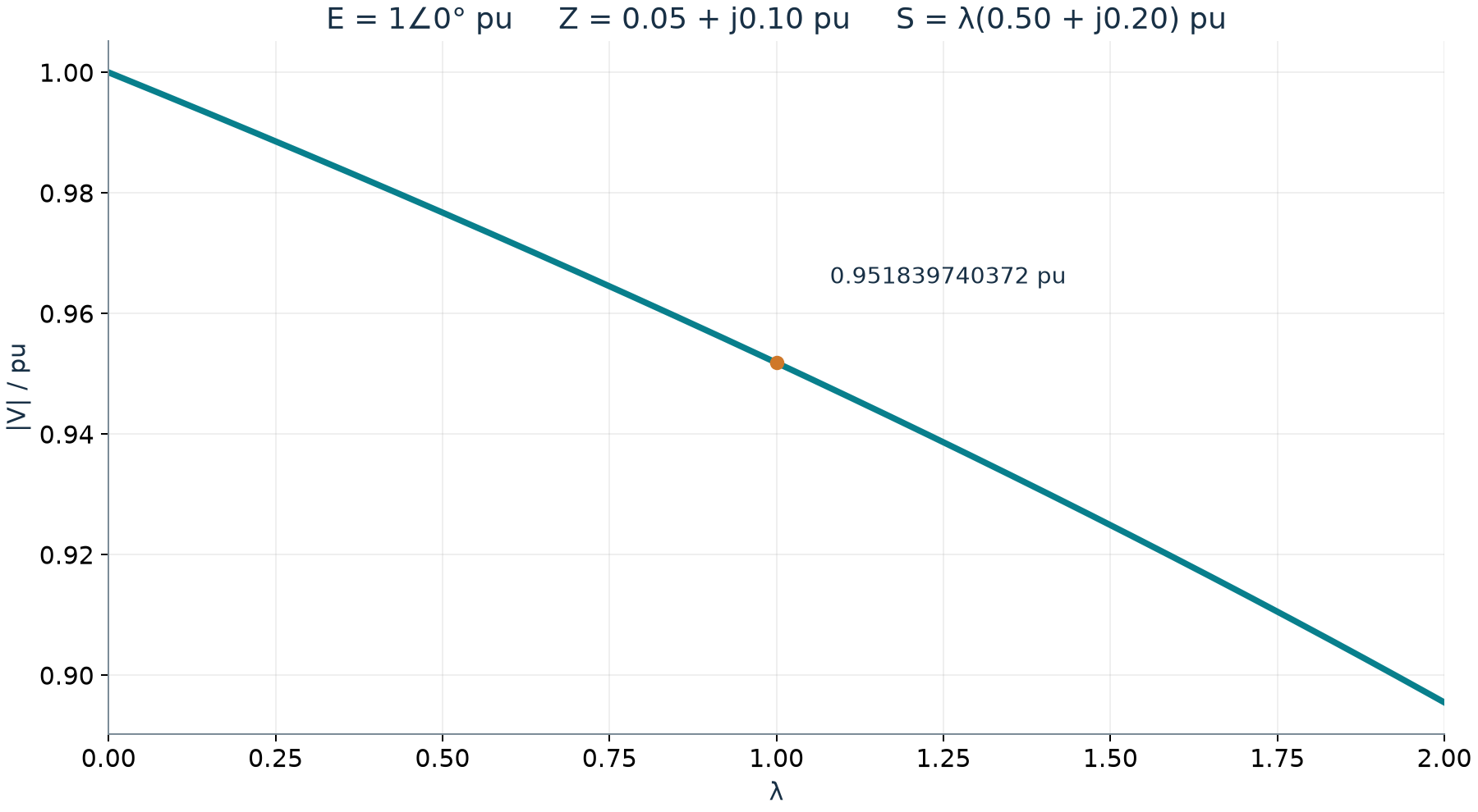
Programmatically calculated higher-voltage solution of the declared two-bus case as load multiplier λ changes; not field data or a stability approval.